The lab is live at heat-metrics-lab.pages.dev. Eight chapters, four SVG diagrams, a divergence map across 1,140 cells, and a Phase 1 drift gate that says the JavaScript and Python implementations agree within 0.009 °F across every reference case. Chapter 7 is the interactive centerpiece — the chapter where the reader stops consuming the argument and starts driving it. It’s also the chapter that ended up being two things: a manual sandbox with four sliders, and a live panel that reaches out to api.weather.gov and brings back the three numbers for Phoenix or Houston or wherever the reader wants.

The chapter is at heat-metrics-lab.pages.dev/#chapter-7. This post is the engineering story behind the build.

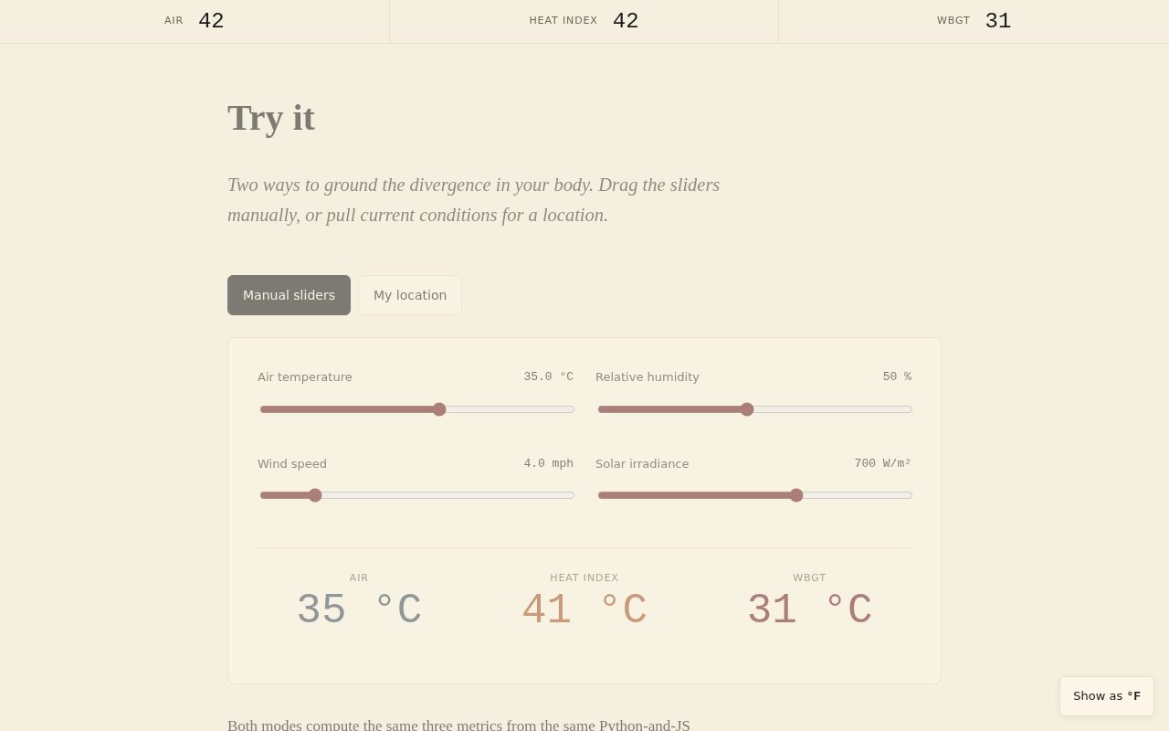Chapter 7 in manual mode. Four sliders, three computed numbers, one set of formulas. The persistent strip at the top of the viewport stays in sync with the chapter’s current reading regardless of which mode is active.

Four things from the build were worth a post on their own.

The dual-mode centerpiece

Most science explainers that include an interactive figure settle for one of two shapes. Either they give you sliders to manipulate — dial the inputs, watch the outputs, develop intuition. Or they give you a location lookup — type a city, see current conditions. Chapter 7 has both, and that’s a deliberate design choice, not scope creep.

The sandbox is the controlled experiment. Hold air temperature at 35 °C and slide RH from 20% to 80%. Heat index moves dramatically — from near parity with air temperature at low humidity to ten-degree overshoot at high humidity. WBGT moves, too, but more modestly. Humidity dominates Heat Index; WBGT is more resistant to it because WBGT’s outdoor form has a wind term and a solar term that don’t touch the psychrometric path. The sandbox makes this legible in about fifteen seconds. You can’t get that from a nomogram or a prose explanation; you need the sliders.

The live panel grounds the chapter in a real place at a real time. Without it, the reader who just wants to know “what’s the WBGT in Phoenix right now” has to leave the page to find out — and they probably won’t come back. The panel closes that gap at the cost of one network request on explicit user action.

Both modes are surfaced through a <div class="ch7-mode-toggle" role="tablist"> element in the markup:

<!-- Ch 7 — Try it (sandbox + live NWS). All three live. -->
<section class="chapter chapter--centerpiece" data-chapter="7" data-act="application" data-metric="all"
         data-readings='{"air_temp_c":35,"hi_c":40.6,"wbgt_c":27.8}'>
  <div class="chapter__inner chapter__inner--centerpiece">
    <h2 class="chapter__title">Try it</h2>
    <p class="chapter__lede">Two ways to ground the divergence in your body. Drag the sliders manually, or pull current conditions for a location.</p>
    <div class="ch7-mode-toggle" role="tablist" aria-label="Calculator mode">
      <button type="button" role="tab" aria-selected="true"  data-mode="manual"   class="is-active">Manual sliders</button>
      <button type="button" role="tab" aria-selected="false" data-mode="location">My location</button>
    </div>
    <div id="sandbox"  data-component="sandbox-calculator"></div>
    <div id="live-nws" data-component="live-nws-panel" hidden></div>

The tab toggle swaps the hidden attribute between the two component containers; both components are initialized at page load and then shown or hidden. When either component produces a reading, it dispatches a chapter-active event onto window:

window.dispatchEvent(new CustomEvent("chapter-active", {
  detail: {
    chapter: "7",
    metric: "all",
    readings: {
      air_temp_c: state.air_temp_c,
      hi_c: computeHi(),
      wbgt_c: computeWbgt(),
    },
  },
}));

The persistent three-number strip that’s been visible since Chapter 1 picks this up via a window.addEventListener("chapter-active", ...) in src/main.js and re-renders its current readings. The strip doesn’t know which component fired the event; it just reads the payload. Both modes feed the same display surface.

Both components use the playground skill’s single-state-object pattern. There is one plain JS object holding all inputs, with typed defaults. Sliders write into that object. The object is the only argument passed to src/metrics.js. localStorage persists the object on every change. Preset chips load named snapshots into the object, overwriting the current state. The pattern fits an exploratory scientific UI precisely because it’s flat and inspectable — in DevTools you can log the full state at any point and see exactly what the formulas are operating on. There’s nothing hidden in a prop tree or a hook closure.

From src/components/sandbox-calculator.js:

const state = {
  air_temp_c: 35,
  rh_pct: 50,
  wind_mph: 4,
  solar_w_m2: 700,
};

Every slider input event writes one key, persists the object, rerenders the readout. The formula calls are two lines:

function computeHi() {
  return heatIndexC(state.air_temp_c, state.rh_pct);
}
function computeWbgt() {
  if (state.solar_w_m2 <= 0) return wbgtIndoorC(state.air_temp_c, state.rh_pct);
  return wbgtOutdoorC(state.air_temp_c, state.rh_pct, state.wind_mph, state.solar_w_m2);
}

The same heatIndexC, wbgtIndoorC, wbgtOutdoorC exports from src/metrics.js that the Phase 1 drift gate validates against Python. Same module, same exports, one source of truth.

The ZIP→lat/lng pivot, and why the constraint held

Phase 5’s original task description for live-nws-panel.js read:

Reuse the user’s input as either ZIP (geocoded via Open-Meteo’s free geocoding-api.open-meteo.com no-auth endpoint — but check the CSP allowlist and add it if so) or raw lat/lng pair.

The implementer dispatch (Dispatch L, Phase 5 DEVREL.md) caught the conflict immediately. The project’s _headers file contains:

Content-Security-Policy: default-src 'self'; style-src 'self' 'unsafe-inline'; script-src 'self'; img-src 'self' data:; connect-src 'self' https://api.weather.gov; font-src 'self'; base-uri 'self'; form-action 'self'; frame-ancestors 'none'

One external host in connect-src. The hard constraint in CLAUDE.md is “no third-party services / api.weather.gov only.” Adding geocoding-api.open-meteo.com would lengthen that list by one host and directly contradict the stated constraint. The task spec even flagged it as a conditional: “check the CSP allowlist and add it if so.” The implementer read that, looked at the constraint, and chose not to add it.

The pivot: drop the geocoder entirely. The component takes lat/lng directly. Two preset chips cover the likeliest demo scenarios:

const PRESETS = [
  { label: "Phoenix, AZ", lat: 33.45, lng: -112.07 },
  { label: "Houston, TX", lat: 29.76, lng: -95.37 },
];

A reader who wants their own coordinates can pull them from Google Maps in two clicks and paste them in. The input accepts any lat, lng decimal string. The parse function is a ten-line regex + range check that accepts common separators and rejects anything outside the WGS-84 bounds.

This is strictly less convenient than a ZIP code box. The honest framing is: the project shipped v1 with a lat/lng input because the cost of the convenience improvement (a new external dependency, a wider CSP surface) wasn’t worth the benefit at this stage. The constraint exists because every entry in connect-src is a domain the browser is willing to send credentials-bearing requests to, and keeping that list short is a security posture, not a formality. The implementer respecting the constraint rather than rationalizing around it is the right outcome.

The two-stage api.weather.gov fetch

NWS doesn’t have a GET /conditions?lat=33.45&lng=-112.07 endpoint. Its data is organized by forecast office and grid cell; lat/lng is the key into a resolver, not the key into the forecast. That means every fetch is two requests.

Stage 1: resolve the gridpoint.

const pointResp = await fetch(
  `https://api.weather.gov/points/${lat.toFixed(4)},${lng.toFixed(4)}`,
  { headers: { Accept: "application/geo+json" } }
);
if (!pointResp.ok) throw new Error(`NWS /points responded ${pointResp.status}`);
const point = await pointResp.json();
const forecastUrl = point?.properties?.forecastHourly;
if (!forecastUrl) throw new Error("NWS response missing forecastHourly URL");

The /points/{lat},{lng} endpoint returns a GeoJSON feature whose properties.forecastHourly field is the actual URL for that location’s hourly forecast — something like https://api.weather.gov/gridpoints/PSR/167,52/forecast/hourly for Phoenix, where PSR is the Phoenix forecast office and 167,52 is the grid cell. You can’t construct that URL from a lat/lng without the first request.

Stage 2: fetch the forecast.

const fcResp = await fetch(forecastUrl, {
  headers: { Accept: "application/geo+json" }
});
if (!fcResp.ok) throw new Error(`NWS forecastHourly responded ${fcResp.status}`);
const fc = await fcResp.json();
const periods = fc?.properties?.periods;
if (!Array.isArray(periods) || periods.length < 1)
  throw new Error("NWS forecast was empty");

const current = periodToReading(periods[0], lat);
const forecast = periods.slice(0, 6).map(p => periodToReading(p, lat));

The hourly forecast returns up to 156 periods (roughly a week out). The component takes periods[0] as the current-hour reading and periods[0..5] as the six-hour forecast. Each period is passed to periodToReading, which handles four conversions:

Temperature. NWS returns Fahrenheit when temperatureUnit === "F". The conversion is exact: (p.temperature - 32) * 5 / 9.

Relative humidity. NWS exposes relativeHumidity.value when it has a direct observation; otherwise it gives dewpoint.value in Celsius. When RH isn’t directly available, the component falls back to the Magnus formula approximation:

const a = 17.625, b = 243.04;
const es_t  = Math.exp((a * temp_c) / (b + temp_c));
const es_td = Math.exp((a * td)     / (b + td));
rh = Math.min(100, Math.max(5, 100 * es_td / es_t));

Constants a = 17.625, b = 243.04 are the August-Roche-Magnus coefficients. The min(100, max(5, ...)) clamps prevent physically impossible RH from cascading through the heat-index formula.

Wind speed. NWS encodes wind speed as a string like "5 mph", "10 to 15 mph", or occasionally "10 km/h". The component pulls the leading number with a regex and converts km/h to mph when the unit suffix indicates it. The fallback when the string can’t be parsed is 4 mph — a light breeze, not zero, because a zero-wind WBGT outdoor calculation with high solar would spike unrealistically.

Unit conversion for src/metrics.js. The formula module works in Celsius and mph (matching the Phase 1 drift-gated reference cases). Temperature is already in °C after the first conversion; wind stays in mph because the outdoor WBGT formula was calibrated that way. No further conversion needed.

The six-hour mini-chart is inline SVG, generated in renderChart:

const series = [
  { key: "air_temp_c", color: "var(--air)",        label: "Air"  },
  { key: "hi_c",       color: "var(--heat-index)",  label: "HI"   },
  { key: "wbgt_c",     color: "var(--wbgt)",        label: "WBGT" },
];

Three <path> elements, one per metric, plus endpoint dots at periods[5] with text labels. The viewBox is 0 0 480 140. Hour labels (+0h, +3h, +5h) along the x-axis. No chart library; no dependency. The whole renderer is about 60 lines of SVG string generation. Pulling in Chart.js or d3 to draw three lines on a 480×140 canvas would cost 300+ KB of dependency and require a bundler, which this project deliberately doesn’t have. The no-bundler discipline (same discipline as DecompressionStream in heat-protein-lab) is one rule that holds across every chapter: if you can write it in thirty lines of vanilla JS, you write it in thirty lines of vanilla JS.

Error handling at the component level is honest rather than opaque: NWS responds with an HTTP 400 (and a detail field explaining the error) when the coordinates are outside NWS coverage. Phoenix and Houston work. Hawaii works. Lytton, BC does not — NWS only covers the contiguous US, Alaska, and Pacific territories. The error path sets state.error = "Couldn't reach NWS: ${err.message}. Try Manual mode instead." and renders it inline rather than silently breaking.

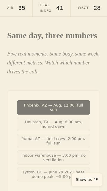The Chapter 4 scenario flipper at mobile width, which uses the same playground-pattern state object as Ch 7’s sandbox. The SVG charts in both chapters use width="100%" preserveAspectRatio="xMidYMid meet" — no fixed pixel widths in the rendered attributes, so they scale cleanly to any viewport without media query surgery.

The solar-elevation estimator

NWS reports cloud cover (0–100%) per period in skyCover.value. It doesn’t report direct solar radiation. To compute an outdoor WBGT, you need solar irradiance in W/m². The component estimates it from two ingredients.

Solar elevation angle. A simplified NOAA SOLPOS-style calculation from latitude, day-of-year, and local hour-of-day:

function solarElevationAt(isoString, lat) {
  const d = new Date(isoString);
  if (Number.isNaN(d.getTime())) return 30;
  const dayOfYear = Math.floor((d - new Date(d.getFullYear(), 0, 0)) / 86400000);
  // Solar declination
  const decl = 23.44 * Math.sin((2 * Math.PI * (dayOfYear - 81)) / 365);
  const localHour = d.getHours() + d.getMinutes() / 60;
  // Hour angle: 0 at solar noon (approximated as local noon)
  const hourAngle = 15 * (localHour - 12); // degrees
  const sinElev = Math.sin(lat * Math.PI / 180) * Math.sin(decl * Math.PI / 180)
                + Math.cos(lat * Math.PI / 180) * Math.cos(decl * Math.PI / 180)
                  * Math.cos(hourAngle * Math.PI / 180);
  return Math.max(-90, Math.min(90, Math.asin(sinElev) * 180 / Math.PI));
}

The declination formula — 23.44 * sin(2π * (dayOfYear - 81) / 365) — is the same approximation used in NOAA’s online calculator and in most clear-sky radiation models accurate to a degree or two. The dayOfYear - 81 offset aligns the sine curve with the vernal equinox (roughly March 22, day 81). The hour-angle approximation treats local clock noon as solar noon, which is off by up to ±30 minutes depending on where within a time zone the location falls. That error propagates to roughly ±2° in elevation at low angles.

Cloud-cover scaling. Given elevation angle elevDeg and cloud cover fraction cloudFrac = sky_cover_pct / 100:

const sinElev = Math.max(0, Math.sin(elevDeg * Math.PI / 180));
const solar_w_m2 = Math.max(0, 1000 * sinElev * (1 - 0.7 * cloudFrac));

At solar elevation elevDeg, the clear-sky peak at sea level is approximately 1000 * sin(elevDeg) W/m². Cloud cover attenuates it by a factor of (1 - 0.7 * cloudFrac). At summer-solstice midday in Phoenix (lat 33.45°), solar elevation reaches roughly 80°, giving a clear-sky estimate of about 985 W/m². At 50% cloud cover that falls to roughly 640 W/m². Fully overcast (100% sky cover), the same midday scenario yields about 295 W/m². Dawn or dusk, elevation near zero, the estimate bottoms out near zero. When the estimate is exactly zero, the component uses wbgtIndoorC instead of wbgtOutdoorC and labels the WBGT reading accordingly.

The chapter body text is explicit about what this is:

“In location mode, NWS doesn’t directly report solar — we approximate it from cloud cover plus the sun’s elevation at your time and place. That’s an estimate, not a measurement. An actual jobsite reading would come from a calibrated WBGT meter sited per ISO 7243. The site reading is what matters for compliance; this panel is for orientation.”

The aside.side-dispatch in Ch 7 makes the same point more sharply:

“Your inspector’s reading at your jobsite will not match this. NWS observations are sited per WMO standard — 5 ft above ground, shaded, ventilated, away from radiant surfaces. Your jobsite WBGT measured per ACGIH may differ by several degrees, depending on what surface the worker is standing on, what they’re wearing, and how much radiant load the local environment is throwing at them. The site reading is what counts for compliance.”

Those disclaimers are doing real work. The solar estimator is good enough to distinguish “it’s 4 am and there is no solar load” from “it’s noon in Phoenix in August and the solar load is significant”. That’s all it claims to do. A WBGT meter sited per ISO 7243 with a Bowen-ratio-corrected globe thermometer produces a different number and that number is the one that matters for a §3395 compliance defense.

Beyond the solar approximation itself, there are larger sources of uncertainty in this panel: the NWS gridpoint is a 2.5 km grid cell. A location within one kilometer of a coastline, a canyon wall, or a dense urban heat island may differ measurably from the gridpoint center. The panel surfaces the NWS reading at the nearest gridpoint; it doesn’t model microclimate deviation. That’s documented in the UI copy and it’s why the disclaimer language says “orientation,” not “site measurement.”

Three things I’d do differently

The mode toggle is functional but not a strict tablist. aria-controls isn’t wired to the two panels, so screen-reader announcement when you switch modes is less rich than a proper ARIA tabpanel pattern. The Phase 6 a11y audit (Playwright-driven) caught this as a should-fix. The focus ring works; the role="tab" + aria-selected attributes are present; but the forward pointer from tab to panel is missing. v1.0.1 candidate.

Houston early-morning labels “WBGT (indoor)” correctly but confusingly. When solar_w_m2 === 0 — which happens at dawn in Houston because the sun hasn’t cleared the horizon — the component routes through wbgtIndoorC and labels the output accordingly. That’s mathematically correct: when there’s no solar load, indoor and outdoor WBGT converge anyway. But a reader who opens the panel at 6 am and sees “WBGT (indoor)” might reasonably wonder why the location panel is showing an indoor reading. A label like “WBGT (no solar load)” with a tooltip explaining the formula choice would be clearer.

The six-hour chart has no y-axis ticks. Three lines diverge across the panel, endpoint labels show the final values, but there’s no scale on the left edge. The reader has to read relative divergence, not absolute magnitude. For the purposes of a six-hour trend, relative divergence is probably what matters — but axis ticks at two or three temperature reference points (say, 32.2 °C WBGT, which is the NIOSH ceiling for any work intensity) would make the chart directly actionable. Also v1.0.1.

What this connects to

Chapter 7 doesn’t stand alone. The drift gate from Phase 1 is what makes the “same formulas” claim credible — if you want the story of how the gate was built and what the advisor caught before any formula code shipped, that’s “A 0.5 °F drift gate, and the advisor that caught the formula bug”. The divergence map in Chapter 5 that the tufte-viz skill caught mis-normalized is in “When a chart-critique skill catches a design bug before ship”. The full project announcement with word count and architecture overview is “Heat Metrics Lab is live”. The A/B comparison against heat-protein-lab (Antigravity 2.0 + Google Science Skills vs Claude Code + Anthropic ecosystem) is “Same brief, two toolchains”.